16 Sample strategies/models using IB-Matlab

16.1 Pairs trading

16.1.1 Once a day – decide whether two securities are co-integrated 171

Download http://www.spatial-econometrics.com/ (jplv7.zip) and unzip into a new folder (this is a free alternative to Matlab’s Econometrics Toolbox172).

Add the new toolbox function to your Matlab path. Naturally, use the actual folder name where you’ve unzipped the toolbox rather than my C:\... example:

addpath(genpath('C:\SpatialEconometricsToolbox'));

Use IB-Matlab to get last year’s daily history data for both securities:173

IBM_history = IBMatlab('action','history', 'Symbol','IBM', ...
'DurationValue',1,'DurationUnits','Y',...
'BarSize','1 day');

GOOG_history = IBMatlab('action','history', 'Symbol','GOOG', ...
'DurationValue',1,'DurationUnits','Y',...
'BarSize','1 day');

% Transform row vectors => column vectors for the adf,cadf tests
IBM_close_prices = IBM_history.close'; % array of 252 values GOOG_close_prices = GOOG_history.close'; % array of 252 values

Ensure that both time series are not already stationary (do not have a unit root and tend to mean-revert). This is done with the adf (Augmented Dickey-Fuller test) function in the Spatial Econometrics Toolbox, which outputs a results struct that enables us to determine at varying confidence levels if this is in fact the case. ADF has the null hypothesis that the time series has a unit root and is non-stationary. To reject this, the absolute value of results.adf (the t-statistic) needs to be greater than the desired absolute value of results.crit – a vector that contains 6 confidence level values, corresponding to 99%, 95%, 90%, 10%, 5% and 1% confidence. Only if the null hypothesis of a unit root and non-stationarity cannot be rejected for both time series in a possible pair, will it be worth proceeding to the cointegration test in step 5.

adfResults = adf(IBM_close_prices,0,1);
if abs(adfResults.adf) < abs(adfResults.crit(3))
% failed test – bail out
end

…and similarly test the second security (GOOG_close_prices here). Note that adf is a necessary but weak test: most securities will pass this test.

The cadf (Cointegrating Augmented Dickey-Fuller test) function in the Spatial Econometrics Toolbox tests for cointegration between a dependent time series (y) and an explanatory time series (x).174 The results struct output by cadf also includes a results.adf (t-statistic) value and six results.crit values. The null hypothesis here is that the time series are not cointegrated, so to reject this in favor of the pair possibly being cointegrated, the absolute value of results.adf needs to be greater than the desired results.crit value.

cadfResults = cadf(IBM_close_prices, GOOG_close_prices, 0,1);
if abs(cadfResults.adf) < abs(cadfResults.crit(3))
% failed test – bail out
end

NOTES:
There are numerous ways of calculating the beta of the relationship (and how frequently to adjust this) between the y and x time series (IBM and GOOG respectively in the example above) in order to determine the correct relative number of shares to buy/sell in each stock in a cointegrating pair.175

Also, the above tests do not indicate which stock informationally leads the other and which is the dependent/independent variable. Tests such as Granger Causality are intended for this purpose.176

If any of the securities failed any of the above tests, bail out

Compute the correlation factor β between the time series (e.g., using ols):

res = ols(IBM_close_prices, GOOG_close_prices); % β == res.beta

Store STD = std(Closesec1 – β*Closesec2) for later use in the runtime part below

modelData.std = std(IBM_close_prices – res.beta*GOOG_close_prices);

Use IB-Matlab to stream quote data for the two securities:177

modelData.ids(1) = IBMatlab('action','query', 'Symbol','IBM', ...
'QuotesNumber',inf);
modelData.ids(2) = IBMatlab('action','query', 'Symbol','GOOG', ...
'QuotesNumber',inf);

Use IB-Matlab to attach our user-defined callback processing function:178

IBMatlab('action','query', 'Symbol','GOOG', ...
'CallbackTickPrice',{@IBMatlab_CallbackTickPrice,modelData});

16.1.2 Runtime – process TickPrice streaming-quote events

% Callback function to process IB TickPrice events
function IBMatlab_CallbackTickPrice(ibConnector, eventData, modelData)

persistent lastPrice1 lastPrice2

% If this is an event about the BID field of the new tick
if (eventData.field == 1) % == com.ib.client.TickType.BID

if (eventData.price > 0) % disregard invalid values

% Update the security's stored last price with the new info
if (eventData.tickerId == modelData.ids(1))
lastPrice1 = eventData.price;
ignoreFlag = false;
elseif (eventData.tickerId == modelData.ids(2))
lastPrice2 = eventData.price;
ignoreFlag = false;
else
% ignore – not one of the requested pair of symbols
ignoreFlag = true;
end

% Check whether the monitored securities have diverged
% from their steady-state prices in either direction
if ~ignoreFlag && ~isempty(lastPrice1) && ~isempty(lastPrice2)

% Compute the divergence from the steady-state model
deltaPrice = lastPrice1 – modelData.beta*lastPrice2;
meanSpread = 0; % see footnote179

% If the securities diverged too much, start trading
if deltePrice < meanSpread -2*modelData.std

% GOOG overbought vs. IBM, so buy IBM, sell GOOG
IBMatlab('action','BUY', 'Quantity',1, 'Type','MKT',...
'Symbol','IBM');
IBMatlab('action','SELL', 'Quantity',1, 'Type','MKT',...
'Symbol','GOOG');

elseif deltePrice > meanSpread + 2*modelData.std

% GOOG oversold vs. IBM, so sell IBM, buy GOOG
IBMatlab('action','SELL', 'Quantity',1, 'Type','MKT',...
'Symbol','IBM');
IBMatlab('action','BUY', 'Quantity',1, 'Type','MKT',...
'Symbol','GOOG');
end

end % if any price has changed
end % if this is a valid price event
end % if this is the tick's BID-field event
end % IBMatlab_CallbackTickPrice

16.2 Using RSI technical indicator

In this section, we use the RSI technical indicator180 as a simple example of automated trading based on indicator value. The examples can easily be adapted to other indicators, or combinations of indicators.

In the following downloadable code,181 we use the MathWorks Financial Toolbox’s rsindex function182 to generate the RSI indicator values. Users who do not have this toolbox can recreate the rsindex function based on RSI’s mathematical definition.

Naturally, any real-life automated trading system would need to employ additional fail-safe mechanisms in the code, to protect against incorrect data, market outages/crashes etc. For example, you might stop the continuous timers if certain data conditions occur, or you might add stop-loss trading orders. The code below only shows a bare-bones implementation, in order to show how IB-Matlab could be used.

If you need assistance in adapting the code for your specific needs, contact us for a consulting offer.

function [hAxes, hTimer] = IBMatlab_AlgoRSI(varargin)
% IBMatlab_AlgoRSI - simple Price-RSI plot and trading algo
%
% Inputs: list of IBMatlab parameters e.g. 'Symbol', 'Exchange',
% 'Currency', 'BarSize', 'Quantity', 'AccountName', etc.
% Processing: Display interconnected plots of price vs. RSI
% Output: hAxes - handles to plot axes
% hTimer - handle to the update timer object
% Example: IBMatlab_AlgoRSI('Symbol','EUR', 'SecType','cash',
% 'Exchange','idealpro', 'Quantity',100);

% Ensure that we have all mandatory input params
IBMatlab_params = varargin;
symbolIdx = find(strcmpi(IBMatlab_params,'symbol')) + 1;
if isempty(symbolIdx)
error('IBMatlab:NoSymbol','Symbol must be specified!');
end
symbol = upper(IBMatlab_params{symbolIdx});
tagStr = ['RSI_' symbol];

% Prepare the GUI window
hAxes = prepareGUI();
lastAction = '';

% Prepare a timer to periodically check market conditions
period = 60; % [seconds]
hTimer = timer('ExecutionMode','fixedRate', 'Period',period, ...
'Name',tagStr, 'Tag',tagStr, ...
'TimerFcn',@timerFcn);
start(hTimer);

% Prepare GUI window
function hAxes = prepareGUI()
% Create a new figure window for this symbol
titleStr = ['Price / RSI for ' symbol];
figure('NumberTitle','off', 'Name',titleStr, ...
'Tag',tagStr, 'CloseRequestFcn',@closeFig);
zoom on;

% Prepare the plot axes
hAxes(1) = axes('Units','norm', 'Pos',[.1,.50,.87,.45]); %prices
hAxes(2) = axes('Units','norm', 'Pos',[.1,.25,.87,.20]); %RSI
hAxes(3) = axes('Units','norm', 'Pos',[.1,.05,.87,.15]); %open

% Link the X axes of the plots
linkaxes(hAxes,'x');
end

% Callback function upon closing the figure window
function closeFig(hFig, eventData)
try stop(hTimer); delete(hTimer); catch, end
delete(hFig);
end

% Get the latest historical/intraday data from IB
function data = getData()
% Get the historical/intraday data bars from IB
% Note: IBMatlab_params are persisted in the parent function
bars = IBMatlab('Action','history', 'BarSize','5 mins', ...
'DurationValue',1, 'DurationUnits','W', ...
'WhatToShow','MIDPOINT', IBMatlab_params{:});

% Ensure that enough data is available, otherwise bail out
if length(bars.close) <= 15
error('IBMatlab:NoData','Not enough data points!');
end

% Determine the RSI values for the retrieved data
% rsindex() requires a column vector, so transpose the data
RSI_vector = rsindex(bars.close');

% Create timeseries objects for plotting
data.times = datestr(datenum(bars.dateTime, ...
'yyyymmdd HH:MM:SS'));
data.ts_close = timeseries(bars.close, data.times);
data.ts_rsi = timeseries(RSI_vector, data.times);
end

% Trade based on the retrieved IB data
function data = tradeData(data)
% Initialize the data points and trade action
RSI_vector = data.ts_rsi.Data;
openPos = zeros(1,length(RSI_vector));
action = '';

% Get the requested trading quantity
quantityIdx = find(strcmpi(IBMatlab_params,'quantity'))+1;
if isempty(quantityIdx)
quantity = 1;
else
quantity = IBMatlab_params{quantityIdx};
end

% Calculate the trading indicator signals
for idx = 2 : length(RSI_vector)
currentRSI = RSI_vector(idx);
lastRSI = RSI_vector(idx-1);

% If position is open
if openPos(idx-1) ~= 0
% If RSI has crossed 50
if (currentRSI-50)*openPos(idx-1) > 0
% Close the open position
if openPos(idx-1) > 0
action = 'Sell';
else
action = 'Buy';
end
openPos(idx) = 0;
else
% Else, do nothing for now
openPos(idx) = openPos(idx-1);
end

% Else, if RSI>70 going down (overbought reversal?)
elseif currentRSI < lastRSI && currentRSI > 70
% Place a SELL order
action = 'Sell';
openPos(idx) = -quantity;

% Else, if RSI<30 going up (oversold reversal?)
elseif currentRSI > lastRSI && currentRSI < 30
% Place a BUY order
action = 'Buy';
openPos(idx) = quantity;
end
end

% Trade if an action was triggered for latest data bar
if ~isempty(action) && ~strcmp(action, lastAction)
fprintf('%s %sing %d %s\n', ...
datestr(now), action, quantity, symbol);
IBMatlab('Action',action, 'Type','MKT', ...
'Quantity',quantity, IBMatlab_params{:});
end
lastAction = action;

% Add the trading decisions to returned data (for plotting)
data.ts_pos = timeseries(openPos, data.times);
end

% Plot the updated data
function plotData(data)
% hAxes is persisted in the parent function
plotTS(hAxes(1), data.ts_close, 'Closing price', true);
plotTS(hAxes(2), data.ts_rsi, 'RSI', true);
plotTS(hAxes(3), data.ts_pos, 'Open pos', false);
end

% Timer callback function
function timerFcn(hTimer,eventData)
try
data = getData();
data = tradeData(data);
plotData(data);
catch err
disp(err.message);
return;
end
end
end % IBMatlab_AlgoRSI

% Utility function to plot a time-series on an axes
function plotTS(hAxes, data, label, emptyXTicksFlag)
axes(hAxes);
plot(data);
box off;
grid on;
title('');
ylabel(label);
if emptyXTicksFlag
set(hAxes, 'XTick',[]);
end
end

For performance considerations, we can query only the latest market snapshot, or use streaming realtime bars,183 rather than retrieving and processing the entire historical/intraday data series as above. Naturally, this would involve additional code to store the previous data bars and trading decisions. If we use the asynchronous streaming realtime bars mechanism, we could consider replacing the timer callback with a callback on the RealtimeBar event (i.e., set the CallbackRealtimeBar parameter in IBMatlab), to process the bars as soon as they arrive from IB. This is more complex than using a simple timer to query the latest streamed data, of course.

Also note that in the simplistic implementation above, the graphs are cleared and recreated in each timer invocation (every 30 seconds). This implementation can naturally be improved by updating the existing graph’s data instead.184

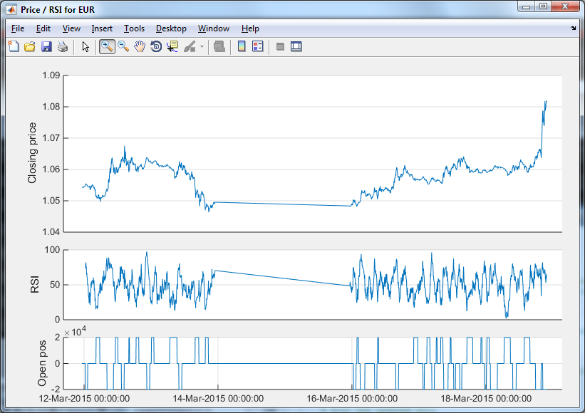
Finally, here is a sample output from running the program for EUR.USD:

>> IBMatlab_AlgoRSI('AccountName','DU12345', 'Symbol','EUR', ...
'SecType','cash', 'Exchange','idealpro', ...
'Quantity',20000, 'BarSize','5 mins');

18-Mar-2015 21:45:01 Selling 20000 EUR
18-Mar-2015 21:53:01 Buying 20000 EUR
...

Sample plotting output of the IBMatlab_AlgoRSI program
(note the trading break over the weekend of 15 March, 2015)

Contact us to receive consulting assistance in building your trading program, based on IB, Matlab and the IB-Matlab connector. We never disclose trading algo secrets used by our clients, so we would not be able to provide you with any actual trading algo that was developed for somebody else. But you will benefit from our prior experience in developing dozens of such trading programs, as well as from our top-class expertise in both Matlab and IB’s API. A small sample of our work can be seen here: http://undocumentedmatlab.com/consulting