Last week, guest blogger Malcolm Lidierth [1] wrote about the open-source Waterloo graphics [2] package and how it can be used in Matlab. Today, Malcolm continues the discussion of Waterloo with a set of examples in Matlab code.
Note: I highly recommend checking out Malcolm’s other open-source submissions/utilities on the Matlab File Exchange [3].
The Waterloo graphics routines provide three potential APIs for MATLAB-users:
- A Java API for the core code provides a simple and consistent mechanism for creating plots using the same data model for each of them, from line and scatter through quiver and contour plots.
- A Groovy API that can be used to call the Java API via some static methods that use Groovy’s dynamic typing mechanisms and so allows the same code to be called with different classes on input from different environments – a cell array from MATLAB for example.
- A Matlab API that mimics the standard MATLAB graphics routines and variously calls the Java-API and Groovy API as required.
I will concentrate here on the Matlab API, which is likely to be of more interest to the majority of readers. This uses Matlab OOP wrappers for the underlying Java objects and all provide access to them by using the getObject() method on the wrappers, so Matlab and Java code can be easily mixed.
Simple Waterloo plots
To create a Matlab figure that can accept Waterloo graphics call GXFigure instead of figure e.g.
f = GXFigure(10);
creates figure 10 and enables it for Waterloo.
In Matlab, you might use gca to create a figure and a set of axes – for Waterloo use gxgca instead. The graph reference also needs to be provided as input to force Matlab to use the Waterloo plotting methods. So
scatter(1:10,1:10,'^r')
in Matlab becomes:
scatter(gxgca, 1:10,1:10,'^r')
Here are the outputs:
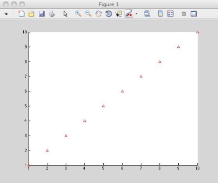
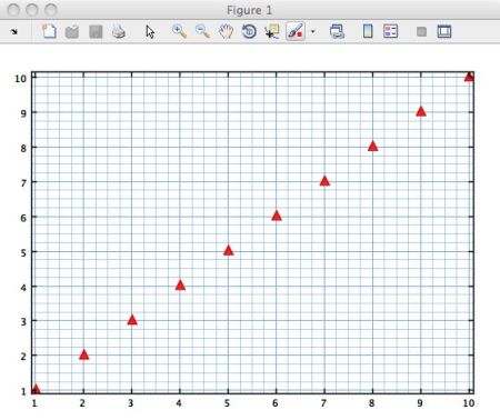
Note that gxgca returns gca if the current axes are not Waterloo-enabled (so its use above would have produced a Matlab scatter plot in that case). If there is no current axes object, it creates a Waterloo
GXGraph and returns a reference to it (just as gca creates Matlab axes when there are none).However, Waterloo does not attempt to completely mimic Matlab: the markers above were specified as ‘^r’. A full LineSpec (e.g., ‘-^r’) would produce an error when given to the scatter function in Matlab, but Waterloo does not care – if a property is specified that is inappropriate it will be ignored. That is because the Matlab properties are translated into a set of Java properties that all plots have in common, but not all plots use. Note also, that hold is effectively ‘on’ for Waterloo, markers are filled and grids are drawn by default (but all the defaults are user-editable).
Combining Waterloo plots
Waterloo plots can be added together. To draw a line through a set of scatter points, a line plot is added to it. Similarly, an error bar plot can be added to that. The Waterloo Matlab-API has an errorbar function that does that. As the plots are additive the process can be continued to create a series of such compound plots:
f = GXFigure();
ax = subplot(f,1,1,1);
set(gcf, 'Units', 'normalized', 'Position', [0.1 0.1 0.8 0.8], 'Name', 'TestError');
x = 0.5 : 0.5 : 10;
y = log(x);
a1 = errorbar(ax, x, y, y/3.5, 'LineSpec', '-ob');
errorbar(a1, [], y*2, y/3.5*2,'LineSpec', '-sg');
errorbar(a1, [], y*5, y/3.5*5, 'LineSpec', '-dr');
Y = errorbar(a1, [], y*10, y/3.5*10, 'LineSpec', '-^m');
ax.getObject().getView().autoScale();
Here I have created a GXFigure, used its subplot method to create a graph, plotted the first errorbar series to it and parented the remaining plots from the first. As they share their x-data, that is specified as empty for the last three plots.
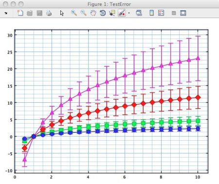
The final line above looks less Matlab-like. For
ax.getObject().getView().autoScale();
axis the Matlab OOP wrapper created by subplot – it’s aGXGraph.- ax.getObject() returns the Java Swing container which has a “view” (which is the graph)
- ax.getObject().getView() returns the graph
ax.getObject().getView().autoScale() just causes the graph to be auto-scaled to fit in all the graphics. The axes can be moved, expanded and shrunk using the mouse and double-clicking displays a GUI editor as shown last week. Clicking on a plot causes the plot to become the current Waterloo graphic object, which can then be accessed with gxgco instead of gco (just as gxgca was used in place of gca).
Combining Matlab and Waterloo sub-plots
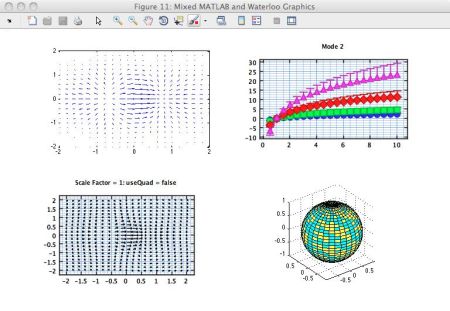
I have shown only single-axes plots till now. The subplot function can, as in Matlab, create multiple axes and these can be used to mix Waterloo and Matlab graphics in a single figure as here (upper-left and lower-right are Matlab):
Some additional examples
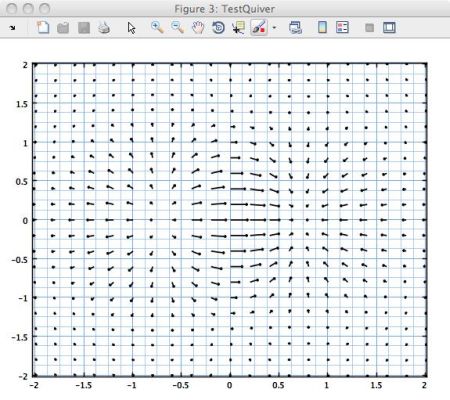
Here then are a few more plot examples:
f = GXFigure();
set(f.Parent, 'Units', 'normalized', 'Position', [.2 .2 .6 .6], 'Name', 'TestQuiver');
[X,Y] = meshgrid(-2:.2:2);
Z = X.*exp(-X.^2 - Y.^2);
[DX,DY] = gradient(Z,.2,.2);
ax = subplot(gxgcf,1,1,1);
q1 = quiver(ax,X,Y,DX,DY, 0.9);
f = GXFigure();
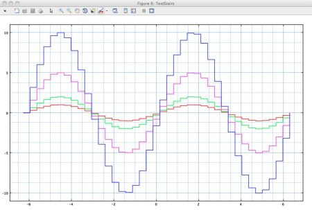
set(gcf, 'Units', 'normalized', 'Position', [0.1 0.1 0.8 0.8], 'Name', 'TestStairs');
x = linspace(-2*pi,2*pi,40);
y = sin(x);
ax = subplot(f, 1, 2, 1);
a1 = stairs(gxgca, x, y, 'LineColor', 'r');
b1 = stairs(gxgca, x, y*2,'LineColor', 'g');
c1 = stairs(gxgca, x, y*5,'LineColor', 'm');
d1 = stairs(gxgca, x, y*10,'LineColor', 'b');
load penny;
f = GXFigure();
ax = subplot(f,1,1,1);
ax.getObject().setAspectRatio(1);  % This sets the aspect ratio of the view in the container
p2 = contour(ax, flipud(P), 30);
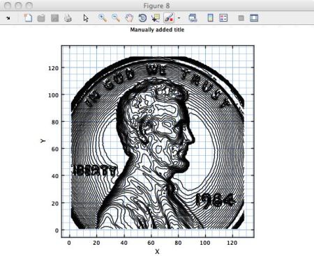
I have added labels and titles here using the GUI editor – they can of course also be set programmatically.
Future work
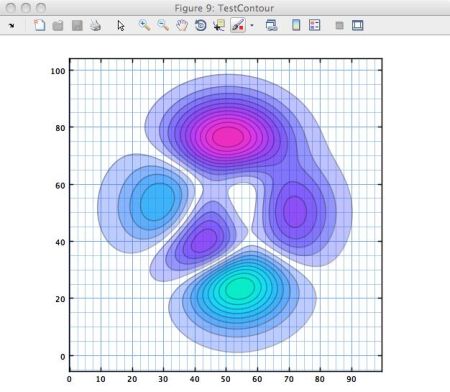
Waterloo is far from finished and more plot types are being added. Here is a taster of a filled contour plot which will be available in the next update (see the development version GIT repository [4]):
f = GXFigure();
set(gcf, 'Name', 'TestContour', 'Units', 'normalized', 'Position', [0.2 0.2 0.7 0.5])
ax = subplot(f,1,1,1);
ax.getObject().setAspectRatio(1);
p1 = contourf(ax, peaks(100), 20);
p1.getObject().setAlpha(0.3);
If you have any comments or feedback on Waterloo, please feel free to join its open-source development effort, or simply leave a comment below [5].
48 Comments To "Waterloo graphics examples"
#1 Comment By Jan On December 7, 2012 @ 06:48
I’ve used older versions of waterloo and quite liked some of the features. Unfortunately I couldn’t deploy waterloo components into MCR delivered applications. Are there any plans to add this capability to waterloo in the future?
#2 Comment By Malcolm Lidierth On December 8, 2012 @ 06:22
@ Jan
I did not have access to MCR until recently. Comments [12] suggest some users have successfully deployed Waterloo components. I do not know enough about MCC/MCR to add anything useful.
#3 Comment By Jan On December 9, 2012 @ 04:40
@Malcolm thanks, I think your comments were what threw me, about waterloo being inherently non-deployable. I missed the comment afterwards about the successful compilation/deployment. From memory the addpath/dynamic class path stuff was not working for me. I didn’t spend much time on it and actually switched to JIDE components and JFreeChart instead.
#4 Comment By Malcolm Lidierth On December 9, 2012 @ 08:17
@Jan
As I understand it, MATLAB copes if you run waterloo.m before doing the MCR build – but you can not call addpath from within a deployed application.
JFreeChart seems excellent. I had a choice when I started this of beginning with JXGraph or building on JFreeChart. I decided on using JXGraph because it was a single class from SwingX and I hope in future to build in features like strip charts using memory mapped buffers as well as supporting 3D graphics using jzy3d. It struck me – maybe wrongly – as easier to start with a relatively blank sheet.
#5 Comment By HAC On December 10, 2012 @ 15:36
Rats, I can’t get it to work via the standalone MCR using 2012b (on Windows 7). It runs in the Matlab environment fine, and seems to compile fine… but when I try running the executable, I get:
I tried re-running waterloo.m just prior to doing the MCR build. No luck.
That’s very unfortunate… Malcolm, if you have any ideas, I’d be glad to test them out.
#6 Comment By HAC On December 11, 2012 @ 06:47
@ Malcolm/Jan:
Okay, so I’ve successfully compiled a deployed application using Waterloo. It turns out that you need to explicitly add the Waterloo source directory to the MCR’s ‘Shared Resources and Helper Files’ list (or use the ‘-a’ command option if you’re compiling via the command line). It appears that it’s not enough to simply ‘addpath‘ and ‘javaaddpath‘ — you’ve got to explicitly point the MCR compiler to the Waterloo directory.
Very exciting! Thanks, Malcolm, for this great resource.
#7 Comment By Malcolm Lidierth On December 11, 2012 @ 08:49
@HAC
Great. I will be looking at MCR delivery in the future so any tips much appreciated.
Malcolm
#8 Comment By Ludvig On December 9, 2012 @ 05:04
Dear Malcolm
Excelent work indeed. I’m wondering about the possibility of combining these plot with the waterloo GUI features, e.g. making the plots in waterloodemo waterloo graphics instead of matlab plots. Is it possible? If so, could you give a simple code example?
#9 Comment By Malcolm Lidierth On December 9, 2012 @ 08:08
@Ludwig
Yes – use GXGraphs instead of a GXFigures. Then you can mix Waterloo and MATLAB graphics in a tabbed pane, accordion etc.
% Create a Tabbed Pane
f=GTabbedPane(figure());

% Waterloo graphics in Tabs 1 & 2
tab1=f.addTab('Tab 1');
tab2=f.addTab('Tab 2');
g1=GXGraph(tab1);
g2=GXGraph(tab2);
p1=scatter(g1,1:10,1:10, 'Color', 'SEAGREEN');
g1.getObject().getView().autoScale();
t= 0:.035:2*pi;
[a,b]=pol2cart(t,sin(2*t).*cos(2*t));
p2=line(g2, a, b, 'LineSpec','-om');
g2.getObject().getView().autoScale();

% MATLAB graphics in Tab 3
tab3=f.addTab('Tab 3');
k = 5;
n = 2^k-1;
[x,y,z] = sphere(n);
c = hadamard(2^k);
surf(x,y,z,c);
colormap([1  1  0; 0  1  1])
axis equal
Waterloo graphics are always housed in a JPanel subclass so they can also simply be added to MATLAB figures/panels using javacomponent or an extension of it – jcontrol from Waterloo or Yair’s uicomponent will both do the job.
If you do not need MATLAB graphics, create a Swing JTabbedPane, JSplitPane etc. Waterloo graphs can be added to those directly.
Regards
Malcolm
#10 Comment By Ludvig On December 9, 2012 @ 12:39
Thanx Malcolm – works great! I tried to plot subplots in a panel, which also seems to work except that a matlab axis keeps showing. Any idea why that is?
GTool.setTheme('green')
f=GTabContainer(figure(), 'top');

% Waterloo graphics in Tabs 1 & 2
tab1=f.addTab('Tab 1');
tab2=f.addTab('Tab 2');

subpanel1 = uipanel('Parent', tab1, 'units','normalized','Position', [0.1 0.1 0.4 0.4], 'BackgroundColor', 'w',...
            'BorderType', 'none');% ,'BorderWidth', 2);
subpanel2 = uipanel('Parent', tab1, 'units','normalized','Position', [0.1 0.55 0.4 0.4], 'BackgroundColor', 'w',...
            'BorderType', 'none');% ,'BorderWidth', 2);

g1=GXGraph(subpanel1);
g2=GXGraph(subpanel2);
#11 Comment By Malcolm Lidierth On December 9, 2012 @ 15:09
GXGraph is less developed/tested than GXFigure and it looks like it can not cope with the nesting here. The generic solution to that would be to use a Waterloo GCGrid (which is what GCFrames use). Sticking as far as possible to MATLAB – use a “wwrap”: that is a generic sibling class of GXGraph that let’s you wrap pretty much any Waterloo container which will then share the same methods as a GXGraph – including MATLAB-style line, scatter etc.
You have a choice – wrap the GJGraphContainer or the GJGraph (I have used the graph below which is the view of the container).
Note also that some things do not work (yet) as with MATLAB-graphics: you can not undock then redock a Waterloo graph from a GTabContainer. That will be easy to fix, but there are a lot of other things to do too.
import kcl.waterloo.graphics.GJGraphContainer;
import kcl.waterloo.graphics.GJGraph;
GTool.setTheme('green')
f=GTabContainer(figure(), 'top');

% Waterloo graphics in Tabs 1 & 2
tab1=f.addTab('Tab 1');
tab2=f.addTab('Tab 2');

subpanel1 = uipanel('Parent', tab1, 'units','normalized','Position', [0.1 0.1 0.4 0.4], 'BackgroundColor', 'w',...
            'BorderType', 'none');% ,'BorderWidth', 2);
subpanel2 = uipanel('Parent', tab1, 'units','normalized','Position', [0.1 0.55 0.4 0.4], 'BackgroundColor', 'w',...
            'BorderType', 'none');% ,'BorderWidth', 2);

g1=jcontrol(subpanel1, GJGraphContainer.createInstance(GJGraph.createInstance()), 'Position', [0 0 1 1]);
g2=jcontrol(subpanel2, GJGraphContainer.createInstance(GJGraph.createInstance()), 'Position', [0 0 1 1]);
g1=wwrap(g1.getView());
g2=wwrap(g2.getView());
line(g1,1:10,1:10);
scatter(g2,1:10,1:10);
#12 Comment By Malcolm Lidierth On December 9, 2012 @ 15:37
@Ludwig
For good measure – here it is using a GCGrid. For good measure I have wrapped that in a GCPanel – as that is currently supported for file saving. Note that the MATLAB figures can not be saved (I have implemented that for GXFigures but for arbitrary nesting of MATLAB uipanels etc that could get difficult). A GCPanel and all of its contents can be saved using:
Here’s the code:
import kcl.waterloo.graphics.GJGraphContainer;
import kcl.waterloo.graphics.GJGraph;
import kcl.waterloo.swing.GCPanel;
import kcl.waterloo.swing.GCGrid;
GTool.setTheme('green')
f=GTabContainer(figure(), 'top');

tab1=f.addTab('Tab 1');
tab2=f.addTab('Tab 2');
panel=jcontrol(tab1, GCPanel(GCGrid(2,1)), 'Position', [0 0 0.5 1]);
g1=panel.add(GJGraphContainer.createInstance(GJGraph.createInstance()));
g2=panel.add(GJGraphContainer.createInstance(GJGraph.createInstance()));
g1=wwrap(g1.getView());
g2=wwrap(g2.getView());
line(g1,1:10,1:10);
scatter(g2,1:10,1:10);
#13 Comment By HAC On December 10, 2012 @ 11:48
Malcolm,
I like what you’ve accomplished, here! Thank you very much for sharing it with the Matlab community.
I’m having a little trouble, though, coming from a MATLAB background with very little Java exposure. For example, how do I simply add X or Y labels to the graph programatically? The xlabel command doesn’t seem to work, and I can’t find the right get/set fields in the axes. In fact, I’d like to do much of what’s available via the Graph Editor GUI on the command line, but I can’t seem to happen upon the right combination of commands.
Furthermore, I’d like to add/edit/remove plotted data programatically — say, update my currently displayed dataset with new values. With normal Matlab axes, I can simply set the axes ‘XData’ and ‘YData’ values. Where do I find the equivalent fields in the GXFigure? I’ve tried poking at some of the exposed methods for the GXGraph class, but seem to have gotten myself lost.
Thanks for your patience!
#14 Comment By HAC On December 11, 2012 @ 07:11
Update: Okay, I think I’ve got some of this worked out. It appears the following will set the x/y labels:
gfig  = GXFigure();
gr1   = subplot(gfig, 1, 1, 1);

gr1.getObject.getView.setXLabel('X Label');
gr1.getObject.getView.setYLabel('Y Label');
So, gr1.getObject() is the Java graph container. I think I’m getting it. I think I can access many of the options found in the Graph Editor GUI such as:
I’m not sure how to set the X/Y limits individually. It’s also not clear to me how to get the current Axis Bounds — it looks like .getAxesBounds comes back with something like:
So, obviously, I can see the [x,y,w,h] values, but I’m not sure how to get them into a Matlab array to manipulate them.
As for my second question (changing X/Y Data on the fly) it appears the answer to this is the .getDataBuffer() method. So, for example, if I wanted to multiply the x-axis data by 0.25, I would do something like:
x = linspace(-10, 10, 100);                         % X Data
y = sin(x./10 .* 2 .* pi);                          % Y Data
data1 = scatter(gr1, x, y);                         % Plot a scatter graph

xdat  = double(data1.getObject().getXData().getDataBuffer()) .* 0.25;
xdat2 = javaArray('java.lang.Double', size(xdat, 1));
for ii = 1:length(xdat)
    xdat2(ii) = java.lang.Double(xdat(ii));
end
data1.getObject().getXData().setDataBuffer(xdat2);
This seems cumbersome — I need to read it in, convert to a Matlab double from a Java double, multiply by 0.25, and then create a javaArray and loop over it to store the data back into a Java-acceptable format. I’m hoping there’s a much easier method of doing this…?
Sorry, I recognize that this is probably very elementary for others; but for me this has been a very fruitful learning exercise!
#15 Comment By Malcolm Lidierth On December 11, 2012 @ 08:11
@HAC
I think you have answered most questions there. A priority is to improve the documenation over the alpha/beta releases.
For the classes you are most likely to need access to, the [13]
To change the data, you do not need to do as much
xdat is a standard MATLAB double. Waterloo does all the needed conversions.Note a couple of related methods
getDataValues: return data transformed by the current axis transform (e.g. log10)
getEntry(index): return the value at the index (zero-based)
setEntry(index,val)
The data buffer returned by getXData()is a GJDoubleDataVector using a java.lang.Double behind the scenes. Get a reference to that with:
changes the data in the plot (i.e. MATLAB workspace and Waterloo are sharing the same array instance).
You do not have to use java.lang.Double: take a look at the kcl.waterloo.graphics.data package.
You can use primitive, double, Double, Float (and BigDecimal!).
In the future, I hope to include a java.nio native backed buffer here too that will allow large data sets from an analog-digital-convertor to be used.
#16 Comment By Malcolm Lidierth On December 11, 2012 @ 08:57
@HAC
As you found, xlabel etc type functionality is exposed but not presently as MATLAB methods following MATLAB naming conventions. If there were demand, that could be included e.g. by providing methods in the MATLAB OOP GXGraphicObject superclass.
For the present, my main aims are [1] to produce proper documentation [2] more plot types.
After that, 3D graphs will be added too using jzy3d.
I do not want to get too distracted with MATLAB – the Graph Explorer needs more work and the GCFrames and GCGrids too. Those work across environments so are not MATLAB specific – and even when used in MATLAB you will notice they are faster and livelier – the Java Swing hierarchy has no MATLAB components.
#17 Comment By Malcolm Lidierth On December 11, 2012 @ 12:02
@HAC
To add/remove plots use the add and remove methods on the graph. Note that adding a plot to a graph, removes it from its present graph if it has one – just as it would with a Swing component. A plot instance can not exist in more than one graph.
#18 Comment By HAC On December 11, 2012 @ 15:06
Thanks for the link to the JavaDocs! I cannot seem to find a reference to ‘kcl.waterloo.plot’… are the docs still a work in progress?
I’m trying to figure out how to change the edge and fill colors for a box created via:
The Java command appears to be (line 63 in annotation.m):
…but I’m struggling to figure out where in the docs I can identify what methods would be available to ‘annot1’ after creation.
#19 Comment By Yair Altman On December 11, 2012 @ 15:24
@HAC – I’m sure Malcolm will point you to the relevant javadoc. But as a general answer to your question, you can see the various methods available to any Java object reference using one of the following Matlab functions: [14], [15], [16] and [17].
#20 Comment By Malcolm Lidierth On December 11, 2012 @ 19:02
@HAC
Yair’s comment is exactly right – all the Waterloo objects can be examined from MATLAB using those methods. Also note, if you are using GXFigures you can fully explore the structure of those using Yair’s findjobj FEX submission.
For the JavaDoc you want kcl.waterloo.annotation.GJAnnotation which is in the ‘base’ library package and on the web-based Javadocs. I realise I need to improve the docs here and get all of them on the web, but there are only so many hours in a day. If you clone the GIT repository you can generate all the JavaDocs in Netbeans.
There is a convention in the naming of classes:
GJ classes are part of the base – always pure Java. These should be stable across releases, so e.g. I will only change the public interfaces if there is a very good reason to from the alpha release and not at all after the full release.
GC classes are higher level containers – used to organise the GJ objects – doing what a MATLAB figure or uipanel does and these are more a work-in-progress.
W classes are Groovy classes that provide wrappers for GJ objects but also, more importantly, static methods that use Groovy dynamic typing to save writing more Java boiler-plate code than needed. Some of the other Groovy code also uses MOP – for example to modify the Groovy Console.
W classes can help to create GJ class objects – but are of no real interest themselves at present. The W class wrappers are not useful in MATLAB because the underlying GJ objects are taken out and wrapped in MATLAB OOP classes. The static methods translate MATLAB properties like LineSpecs into Java properties that the Java code can use – there are many fewer properties in Waterloo than MATLAB because all plots from line and scatter through vector and contour plots share a common data model.
All the packages are in the GIT repo and all can be built with Netbeans. All the Groovy packages can also be loaded in IntelliJ – which provides much better support for Groovy and Scala while the GUIs, like the Graph Editor, have been designed in Eclipse (although often edited in Netbeans) because I much prefer the Eclipse form designer.
The package structure might appear overly complicated, but there is a logic to it. The ‘base’ package for example has dependencies on the ‘gui2’, ‘export’ and ‘widget’ packages. All those dependencies are uni-directional and made via Java interfaces that are implemented in the dependent packages. This means you can use the base library but replace the dependent packages with application-specific custom packages e.g to replace the graph editor with a customised/branded editor for your product by using a replacement for the gui2 package. The widgets package is presently small but provides general purpose widgets. Because there are no circular dependencies, you can include that package in a project that does not otherwise use Waterloo. The same is true for the ‘groovy’ package. I have kept base code written in Java and optional code written in Java in separate projects so you can use Waterloo without bundling Groovy if that is what you need.This structure also lets me provide the code under LGPL but also provide a GPL supplement. The LGPL library provide interfaces that are implemented in the GPL code but there are no class dependencies – and no compile time linking. A link is established only when you install the GPL code and then, in MATLAB, run waterloo.m – so you, rather then me, then create a local GPL instead of LGPL licensed combined work on your PC.
This reply is too long already – so I’ll stop but add that the design is also intended to allow frameworks other than Swing to be supported in the future: JavaFX, Wicket etc. Inevitably, I will not have got all that right – but what I have got right, I hope, will make the job easier.
#21 Comment By HAC On December 12, 2012 @ 07:10
@Malcolm
And thank you for the added explanation. I’m starting to see some of the logic behind the layout. Your efforts, here, are certainly making the Java underbelly of Matlab much more accessible to those of us who currently lack the experience. Thanks!
#22 Comment By HAC On December 12, 2012 @ 07:08
@Yair
Excellent! I was aware of methods(), but not methodsview(). And your contributed uiinspect and checkClass are wonderful! Thanks to both you and Malcolm, I was quickly able to answer my own question about changing the edge/fill colors of my annotation. For completeness:
I appreciate your patience and willingness (both of you!) to teach us ‘how to fish’ and not just ‘catch the fish’ for us.
Much appreciated!
#23 Comment By Malcolm Lidierth On December 12, 2012 @ 08:39
@HAC
Here is some Java:
creates a new immutable Color object instance to use for the color.
uses a reference to the same globally defined static instance of
Color.blackas the rest of the JVM. You don’t need a new instance for every line/letter/border. The memory saving can add up.#24 Comment By HAC On December 12, 2012 @ 09:56
@Malcolm
Ah, that makes sense. And, yes, that will save me a fair amount of memory!
One more question, if I may (forgive me for so many!):
If I create a simple graph…
…and then I view ‘jax’ using Yair’s excellent ‘uiinspect’ function, I see that there are some callbacks available, specifically ‘MouseDraggedCallback’. If I set this callback using familiar Matlab get/set routines, I see:
The callback actually works, but clearly isn’t the right way to do things. According to [18], Yair mentions how it’s best to use the internal Java get/set methods. Alas, there don’t appear to be any appropriate get/set methods for ‘jax’. I tried using the alternatives suggested by Yair in the thread, but I suspect they are only for user data and not actually existing methods.
So… I think I’m getting more self-sufficient, but this one stumps me. 🙂
#25 Comment By Yair Altman On December 12, 2012 @ 12:15
@HAC – the reason for the warning (a memory leak) and the advocated (better) way to set such callbacks is discussed in my article on [19].
#26 Comment By Malcolm Lidierth On December 12, 2012 @ 11:00
@HAC
No need for findjobj here as you have a reference;
gfig = GXFigure();
ax1 = subplot(gfig, 1,1,1);
h=handle(ax1.getView(),'callbackproperties');
set(h, 'MouseDraggedCallback', 'disp(''Mouse drag'')')
Like
Color.black, the mouse listener for all graphs is a static instance and shared by all graphs in a MATLAB session.A caution for Waterloo graphs:
The listening is, in fact, done by the container mouse listener and a “AddedComponentMouseHandler” that pass the mouse events to a graph after a bit of trigonometry to find out what the mouse is over: that is needed because Waterloo lets you rotate and zoom the graphical presentation of the view on screen and Swing knows nothing about that. None of this matters much unless the view is rotated or zoomed.
#27 Comment By HAC On December 12, 2012 @ 11:37
@Malcolm
Beautiful! Thanks very much — and thanks for the warning regarding rotation/scaling in Waterloo. I’m sure that would’ve eventually stumped me!
#28 Comment By Malcolm Lidierth On December 14, 2012 @ 05:54
Fonts could be looked at again. As I recall, the Font for the graph container gets inherited by the other components and I suspect my code is calling setFont after yours and reseting things. I makes sense (to me) to have single font used in a graphical unit.
Fonts can be problematic because the derived Fonts Yair mentions can be platform-specific classes (not just platform-specific Fonts) – problems then de-serializing that data files properly on another platform.
#29 Comment By HAC On December 20, 2012 @ 13:43
It’s not so much the font itself I’d like to change, but the font size and style (bold, italic, etc.). For publishing (as an example), the axes labels and titles are too small.
#30 Comment By HAC On December 13, 2012 @ 05:22
@Malcolm/Yair,
Hmm, so just when I think I’m getting the hang of this, something unexpected happens. It appears that I cannot get some Java methods to respond. For example:
gfig = GXFigure();                                             % Create Figure
ax1 = subplot(gfig, 1,1,1);                                    % Create axes
annot1 = annotation(ax1, 'box', 0, 0, 0.4, 0.4);               % Add Box
ax1.getView.repaint;                                           % Update View
annot1.getAnnotation.getPath.getBounds2D.getMaxX               % This correctly returns 0.4
annot1.getAnnotation.getPath.getBounds2D.setRect(0,0,0.6,0.6); % *** But this doesn't change the box size!
ax1.getView.repaint;                                           % Update View (no effect)

h = handle(ax1.getView);                                       % Grab the View handle
h.setXLabel('Test');                                           % Add a Label to the X-Axis
h.setFont(java.awt.Font('Calibri', java.awt.Font.BOLD, 30));   % *** But this doesn't change the font!
h.revalidate();                                                % Looks like the space around the xLabel changes, but the font does not
h.repaint();                                                   % Update View (no effect)
It seems that the setRect() and the setFont() methods do not actually have an effect (after repainting and/or revalidating).
And Malcolm earlier pointed out that I was creating copies of java.awt.Color() when I probably ought to be referencing existing ones to save memory… I imagine I’m doing the same thing here with the setFont() call — so maybe I’m not doing this correctly at all?
(I’m a scientist pretending to be a programmer. Apparently I have just enough knowledge to be dangerous!)
#31 Comment By Malcolm Lidierth On December 13, 2012 @ 06:37
@HAC
getBounds on a Path returns the bounds of the lineTos, moveTos etc in the Path. You can not change that without operating on the Path object e.g. by scaling/ translating it using an AffineTransform. I doubt anyway that I give you access to the object rather than a copy of it because repeated transformations e.g in the paint routines would scale the same instance every time and so produce nonsense.
For the Font I suspect that is my code ignoring your instruction. Waterloo uses the same font by inheriting it from higher up the Swing hierarchy. This keeps files smaller and means the default font should look OK cross-platform e.g. is Callibri present on Linux/so you want to embed that font in an SVG file etc. This bahaviour can change – that’s the point of an alpha release to see what people want.
#32 Comment By HAC On December 13, 2012 @ 12:45
@Malcolm
Ah, I see. Perhaps a better approach (until Alpha3) is to draw the objects and then delete them and re-draw with my new coordinates.
As for the font, I’m more concerned about controlling the font size than type, so if it’s easier to keep the available font(s) to a list of OS-independent sets (or just a single one), that’s fine for me, personally. But I need to allow the end-user to change the font size.
This idea of a Java font object has me a little confused. If I set a font by using a java.awt.Font() object, can I not modify the individual settings of that particular object (e.g., change the font size, type, or style) without needing to create a new and different font object? The same goes for java.awt.Color() objects. Rather than creating and destroying many Color() objects, can’t I just change the RGB values associated with an existing Color() object?
#33 Comment By Yair Altman On December 13, 2012 @ 15:05
@HAC –
FontandColorare [20] Java objects, so you can’t modify an existing object of these classes.Fonthas a deriveFont() method that you can use to create a newFontobject based on an existing one with some changes, but this still means creating a new object.#34 Comment By Peter On January 21, 2013 @ 09:00
Very nice graphs indeed. However I still struggle to understand some of the basic issues of how everything works. For a simple example, how do I simply replot in a graph, i.e. update the data. I have tried the following:
This updates the data points but the old line remains (same for e.g. errorbar).
I also tried to clear the window, e.g. by calling ax.getObject.getView.removeAll or ax.getObject.getView.removeAllPlots, (followed by autoScale) which does not work or gives a bunch of errors.
I think I get that the plots are objects, i.e. there is no simple “hold on” “hold off” property as in matlab – once you put an object into a graph, it is there so either you have to delete it or manupulate its data to change it, is that correct?
More articles on this excellent tool would be highly appreciated! It takes matlab figures at least 10 years into the future!
#35 Comment By Malcolm Lidierth On January 22, 2013 @ 06:35
Peter
The plots are built up from “primitives” so a line with markers is two plots – a line + a scatter plot. For errorbar plots there are three: a line + a scatter plot + the error bars themselves.
In the MATLAB line method I should perhaps have set the line & scatter to share the underlying data object by reference. Your code would then work and I’ll look at that for the next update. For the present they do not, so you need to update the data for both the line and scatter plot by adding 1 line of code:
Alternatively, you could create the share-by-reference situation thus linking the two plots. Updating either will then update both.
At the MATLAB prompt you will then see:
The underlying data objects have the same hash code – they are the same instance.
The underlying data buffer is a java.lang.Double[]. That too, can be retrieved by reference in MATLAB. That contrasts with a primitive double[] which will always be copied to and from Java as a copy rather than a reference e.g. getRawDataValues passes back a new double primitive array.
The logic for the underlying Java plots is that the line and scatter may need to be separate in some situations e.g if the line is a fitted curve. Also, if an axis is transformed the line will still appear as a straight Java2D primitive line between the data points (effectively then creating a spatial aliasing issue because each line has just two data points). But, by creating e.g. 100 points for the line between each point on a scatter each of the 99 line segments will be transformed – and appear on screen accurately reflecting the applied transform.
#36 Comment By Peter On January 23, 2013 @ 13:57
Malcolm, thanks a lot. I am (slowly) grasping how this thing works. I guess it is a bit harder for those of us comming from a Matlab only background without previous java exposure.
By the way – does your toolbox have anything similar to matlab’s imagesc and text commands? (what I would like to do is to plot a matrix where the cell’s are color coded depending on the corresponding value in the matrix and, at the same time, the cell value is written in the cell).
Thanks again. I realy feel that this package is such a huge improvement over (most) matlabs figures that I will try to invest the time necessary to learn it.
Best Regards
Peter
#37 Comment By Malcolm Lidierth On January 23, 2013 @ 15:53
Peter
Documentation will improve in time. Nothing similar to imagesc yet (although there is an image viewer in the GraphExplorer) but text annotations are available – see the TestAnnotation demo.
I do not understand exactly what you are after. Could you give a MATLAB code snippet to demonstrate?
Malcolm
#38 Comment By Peter On January 24, 2013 @ 11:34
What I was trying to do was visualizing a matrix, i.e. something like this:
In matlab, I have used imagesc, which color-codes whole cells but the above is OK. Then in the center of each square, I would like to have a text with the corresponding value (centered and transparent). The code below does the job but the text is a bit off the center and has a gray background, which is kind of ugly.
for i=1:length(maturities)   % Iterate over X
    for j=1:5
        annotation('Parent', ax, 'Style', 'text', 'XData', i,...
            'YData', j,'Text', num2str(y(i,j),'%0.2f'));
    end
end
ax.getObject.repaint;
I also tried to add som mouse handling events to figures – mouseClicked worked as expected but I couldn’t get mouseDragged to work as intended since the whole waterloo-graphs moves when you click and drag the mouse. Is there anyway to turn this feature off?
Best Regards
Peter
#39 Comment By Malcolm Lidierth On January 25, 2013 @ 06:17
Peter
The colors fonts etc are all editable properties of the underlying java object.
For alignment, I need to add some new methods but the existing
add(component, x, y, alignX, alignY)method in the graph container should be OK (the component will not be added to the list of annotations though so I’ll improve this).
#40 Comment By Malcolm Lidierth On January 28, 2013 @ 03:45
@Peter
I forgot – annotations use graphics not swing so that option is not available. I’ll need to add some code, But here is a solution using JButtons:
gr=ax.getObject().getView();
for i=1:size(X,1)
    for j=1:5
        annot=javaObjectEDT(javax.swing.JButton(num2str(y(i,j),'%0.2f')));
        annot.setPreferredSize(java.awt.Dimension(20,15));
        annot.setFont(java.awt.Font('Arial',java.awt.Font.ITALIC, 8));
        gr.add(annot,i,j,javax.swing.SwingConstants.CENTER,javax.swing.SwingConstants.CENTER);
    end
end
Add callbacks to the buttons directly.
To replace (rather than supplement) the default mouse + mouse motion listeners with MATLAB callbacks, you will need to explicitly remove the existing Java listeners.
#41 Comment By Malcolm Lidierth On January 28, 2013 @ 03:58
PS
might look better as the Swing layout has only 1-pixel resolution.
#42 Comment By Yannick On February 25, 2013 @ 08:51
Awesome work! In no time I was able to implement this into my GUI’s and the plots look so much better.
One question to the more experienced users, is there an easy way to produce a legend with the line and marker properties such as the default in Matlab ?
Thanks!
#43 Comment By Malcolm Lidierth On February 26, 2013 @ 06:28
Yannick
Not yet I am afraid. I hope to post the Alpha3 version soon. That has quite a few new elements: mouse selectable ROIs, area plots, bar charts etc. many from suggestions arising from this blog.
The ROIs (and also a color bar) are there as draggable insets in Alpha3 and I plan to implement a legend that way too.
Regards
Malcolm
#44 Comment By Yannick On February 26, 2013 @ 09:23
Can’t wait for Aplha 3 then !
Thanks again for that awesome piece of work.
#45 Pingback By Waterloo graphics beta | Undocumented Matlab On July 2, 2013 @ 10:01
[…] ended my last guest article with an example of work-in-progress: filled contours. The beta release now fully supports […]
#46 Comment By Ben On August 14, 2013 @ 16:45
Thanks for the beautiful examples.
I’ve installed it and managed to get the examples work but I couldn’t annotate the figure (say with an arrow). This is what I have tried:
Nothing appears…
Can you please show an example of how to annotate with an arrow?
#47 Comment By Shannon Chow On October 29, 2014 @ 04:26
How to enable the “dock” and “close” button in the GTabedPane?
#48 Comment By Wilber On December 26, 2017 @ 23:31
Yair
Am I doing something wrong? I can’t correct the problem. Can you help me please.
This is the code:
f = GXFigure();
set(f.Parent, 'Units', 'normalized', 'Position', [.2 .2 .6 .6], 'Name', 'TestQuiver');
[X,Y] = meshgrid(-2:.2:2);
Z = X.*exp(-X.^2 - Y.^2);
[DX,DY] = gradient(Z,.2,.2);
ax = subplot(gxgcf,1,1,1);
q1 = quiver(ax,X,Y,DX,DY, 0.9);

Attempt to reference field of non-structure array.

Error in subplot (line 43)
set(0, 'CurrentFigure', target.Parent);%figure(target.Parent);%

Error in subplot (line 76)
    ah=subplot(varargin{1:2}, varargin{3});