Waterloo graphics beta

Once again I’d like to welcome guest blogger Malcolm Lidierth of King’s College London. Malcolm has written several articles here, including a couple of articles on his Waterloo graphing library. Today, Malcolm discusses new features in this library, as it matures into an official beta phase.

1. Introducing new plot types: contours, bars, polar and area charts
2. Mouse-selectable regions of interest
3. Support for fast-plot updates without redrawing the entire graph
4. Support for web-deployment of the graphs using SVG or Processing and ProcessingJS

Today I will concentrate on [1] and [2], illustrated with some Matlab examples; I will discuss [3] and [4] next week.

Installation of Waterloo in Matlab

For those readers who have not yet installed Waterloo in Matlab, the process is very simple: download the latest zip file and extract it. All the sub-folders in the waterloo folder are needed but only the Waterloo_MATLAB_Library subfolder (not its subfolders) should be added to the Matlab path. Once installed, just type waterloo at the Matlab prompt in each Matlab session.
A Matlab script file that will do it all is available here (Waterloo_installer.m). The script is harmless to run if you already have Waterloo installed, but if not then it will automatically find the latest zip file on SourceForge, download and install it, and then configure the Matlab path appropriately.

Contour plots

I ended my last guest article with an example of work-in-progress: filled contours. The beta release now fully supports these.
Recall from the previous articles that GXFigure creates a Waterloo-compatible Matlab figure window. gxgca() returns a reference to the container for the graph as a Matlab GXGraph object, much as Matlab’s built-in gca returns an axes reference.
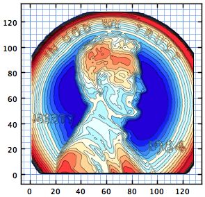
Here is Matlab’s Lincoln penny demo in Waterloo:

% Get some pre-defined colors
colors = [kcl.waterloo.defaults.Colors.getColor(0)];
for k = 1 : 17
    colors = horzcat(colors,kcl.waterloo.defaults.Colors.getColor(k));
end
f = GXFigure();
set(gcf, 'Name','Filled Contour', 'Units','normalized', 'Position',[0.3 0.3 0.4 0.4])
load penny;
ax = subplot(f,1,1,1);
ax.getObject().setAspectRatio(1);
p2 = contourf(ax, flipud(P), 18, 'LineStyle','-', 'LineWidth',0.4);
p2.getObject().setFillClipping(false);
p2.getObject().setFill(colors);
drawnow();

(resulting in the contour plot above)
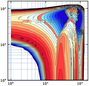
To transform Abe Lincoln to a logarithmic world, just double-click the graph and select the log transform. The result is shown on the right here:

• the data model incorporates an extra object to do the work
• such plots implement a new interface – GJTransformUpdateInterface – that specifies a transformUpdate() method that refreshes the pixel-coordinates. End-users will not normally need to concern themselves with this, as transformUpdate method will be called by the listeners as required.

Categorical data

Waterloo always uses numeric data to position markers, bars etc in a plot. However, categorical data can be used to supplement those data. Here is an example using the new bar plot:

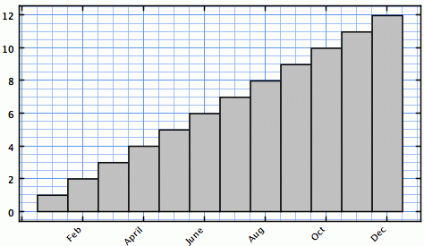
f = GXFigure();
set(gcf, 'Name','TestBar4', 'Units','normalized', 'Position',[0.1 0.1 0.8 0.8]);
m = {'Jan', 'Feb', 'March', 'April', 'May', 'June', 'July', 'Aug', 'Sept', 'Oct', 'Nov', 'Dec'};
gr1 = subplot(f, 2, 2, 1);
a = bar(gr1, 1:12, 1:12);
for k = 1 : 12
   a.getObject().getDataModel().getXData().setCategory(k, m{k});
end
gr1.getObject().setTitleText('Label using the XData categories');
gr1.getObject().getView().autoScale();

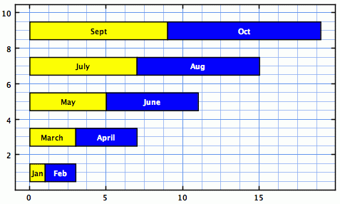
Support for categorical labels on the axes is supported for all plots via the common data model. For bar charts, the extra object associated with the plot also supports adding labels to the bars themselves:

f = GXFigure();
set(gcf, 'Name','Categorized Bars', 'Units','normalized', 'Position',[0.3 0.3 0.4 0.4]);
m = {'Jan', 'Feb', 'March', 'April', 'May', 'June', 'July', 'Aug', 'Sept', 'Oct', 'Nov', 'Dec'};
gr = subplot(f, 1, 1, 1);
c = barh(gr, 1:10, 1:10,'stacked');
c.getObject().setFill([java.awt.Color.yellow, java.awt.Color.blue]);
c.getObject().getDataModel().getExtraObject().setFontForeground([java.awt.Color.BLACK, java.awt.Color.WHITE]);
for k = 1 : 12
   c.getObject().getDataModel().getExtraObject().getLabels().add(k-1, m{k});
end
gr.getObject().getView().autoScale();

Note that the standard method setFill, is used to set the bar colors and as two colors are supplied the data are assumed to contain a pair of multiplexed series. This is common to all plots.
To customize the labels, we need to set a property in the extra object which is retrieved with a call to c.getObject().getDataModel().getExtraObject().
The same principles apply to pie charts:

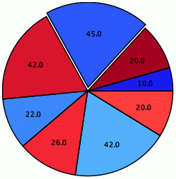
f = GXFigure();
set(gcf, 'Name','TestPie1', 'Units','normalized', 'Position',[0.1 0.1 0.8 0.8]);
colors = [kcl.waterloo.defaults.Colors.getColor(0)];
y = ones(1,18)*100/18;
gr = subplot(f, 1, 1, 1);
colors = [kcl.waterloo.defaults.Colors.getColor(1),...
    kcl.waterloo.defaults.Colors.getColor(17),...
    kcl.waterloo.defaults.Colors.getColor(2),...
    kcl.waterloo.defaults.Colors.getColor(16),...
    kcl.waterloo.defaults.Colors.getColor(3),...
    kcl.waterloo.defaults.Colors.getColor(15),...
    kcl.waterloo.defaults.Colors.getColor(4),...
    kcl.waterloo.defaults.Colors.getColor(14)];
c = pie(gr, [10 20 45 42 22 26 42 20], logical([0 0 1]), 'FaceColor',colors);

Polar charts

Polar bar and compass charts are also now supported:

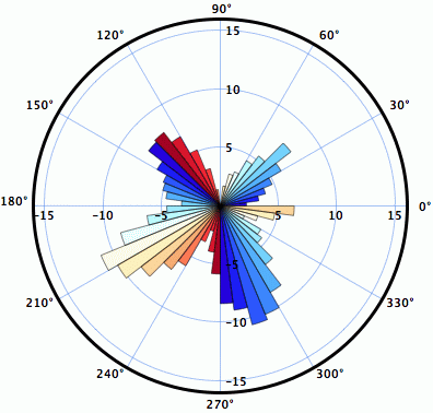
f = GXFigure();
set(gcf, 'Name','TestPie1', 'Units','normalized', 'Position',[0.1 0.1 0.8 0.8]);
load sunspot.dat  % Contains a 2-column vector named sunspot
colors = [kcl.waterloo.defaults.Colors.getColor(0)];
for k = 1 : 17
    colors = horzcat(colors,kcl.waterloo.defaults.Colors.getColor(k));
end
gr1 = subplot(f, 1,2, 1);
a = polarbar(gr1, sunspot(1:48,2), 'FaceColor',colors, 'EdgeWidth',0.5);
[a,b] = hist(sunspot(:,2),12);
gr2 = subplot(f, 1,2, 2);
b = polarbar(gr2, a, 'FaceColor',colors);
Z = eig(randn(20,20));
a = compass(gr1, real(Z), imag(Z), 'LineColor','r');

Area plots

Area plots are supported through a new plot class and also by having all plots implement a new Java interface. To illustrate, create two line plots:

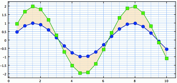
f = GXFigure();
set(gcf, 'Name','TestAreaFill', 'Units','normalized', 'Position',[0.4 0.1 0.5 0.4]);
x = 0.5 : 0.5 : 10;
y = sin(x);
gr1 = gxgca();
a1 = line(gr1, x, y, 'LineSpec','-ob');
b1 = line(gr1, x, y*2, 'LineSpec','-sg');
gr1.getObject().getView().autoScale();
% Filling the area between the two plots requires one extra line and a refresh call to paint the result:
a1.getObject().setAreaFill(b1.getObject());
refresh();

All the work is done in the Java code because plots now implement the GJFillable interface. All that is required is to call the setAreaFill() method on a class implementing GJFillable, specifying another GJFillable as input.
A new java class, GJFill, also implements GJFillable and can be used to fill an area relative to a scalar constant or an arbitrary shape. I have also written a Matlab wrapper class for this (GXFill, see below) but I shall use a Java-based example here.
Whether the fill is made horizontally (from the plot) or vertically (from the axes) can be selected by setting the orientation property of the GJFill instance. This can also be set to arbitrary, in which case we can create a custom fillable area sythesized from java.geom shapes:

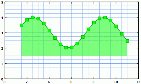
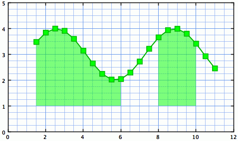
f = GXFigure();
set(gcf, 'Name','Constant Fill', 'Units','normalized', 'Position',[0.3 0.3 0.4 0.4]);
x = 0.5 : 0.5 : 10;
y = sin(x);
gr1 = subplot(f, 1, 1, 1);
a1 = line(gxgca, x+1, y+3, 'LineSpec','-sg');
% Now create a GJFill instance, using a constant as the reference (1.5 in this case), and use this as this area's fill
v = kcl.waterloo.graphics.plots2D.GJFill(a1.getObject(), 1.5);
a1.getObject().setAreaFill(v);
%% Start complex
   % Alternately, we can use an arbitrary fill shape:
   v.setOrientation(javaMethod('valueOf', 'kcl.waterloo.graphics.plots2D.GJFill$ORIENTATION', 'ARBITRARY'));
   a1.getObject().setAreaFill(v);
   % Create a shape (which can be complex)
   area = java.awt.geom.Area(javaObject('java.awt.geom.Rectangle2D$Double',1,1,5,5));
   area.add(java.awt.geom.Area(javaObject('java.awt.geom.Rectangle2D$Double',8,1,2,5)));
   % Add the shape to the GJFill instance
   v.setArbitraryArea(java.awt.geom.Area(area));
%% End complex
% Customize the fill color
v.setAreaPaint(java.awt.Color(0,1,0,0.5));
% Manually rescale and refresh the plot
gr1.getObject().getView().setAxesBounds(0,0,12,5);
refresh();

To make this simpler from Matlab, a new Matlab class GXFill is provided. This constructs and adds a fill in a single step:

fill = GXFill(plot_reference, value, orientation);

where value is a scalar or a Java Shape object, and orientation is a string e.g. ‘horizontal’. Note that the coordinates are specified in axes units and they will rescale and be transformed as needed when the axes are changed.

Specifying/selecting ROIs

Finally, regions of interest (ROIs) can be selected both programmatically and with the mouse. One of these can be set as the “current” ROI and that is the one that is mouse selectable: set the current ROI using shift-left mouse drag, set the region and rescale to display only that region using shift-right mouse drag.
To create an ROI that can be dragged and resized, add a GJRoi instance to the graph, e.g. with an existing current ROI selected:

gr = gxgca;
gr = gr.getObject().getView();
gr.add(kcl.waterloo.graphics.GJRoi.createInstance(gr, gr.getCurrentROI()));

Waterloo and Matlab’s Java support

Note: It appears that HG2, like HG1, creates an offscreen bitmap that is then blitted onto a Java Canvas within a Matlab figure. Matlab warns that the JavaFrame property will (no longer may) be discontinued in some future release, but it is my guess that this will not be the case when HG2 is released. A new set of uicontrols may indeed be included using a C-based library like wxWidgets or Qt. However, it seems unlikely that Java support will be dropped completely – too much of Matlab’s GUI uses Java (for example, the new desktop introduced in R2012b is entirely Java-based). So the Waterloo Matlab library should work, even if a switch is needed to using JFrames instead of Matlab figures for output.
For the adventurous, Waterloo graphs can also be deployed using JavaFX via the SwingNode class – but that requires installation of the latest Java 8 (currently in early release status). Noting that Matlab is still (as of R2013a) using Java 6, this may indeed be a big jump (note last week’s article on upgrading Matlab to use Java 7).
Naturally, Waterloo’s graphs and classes can also be used in stand-alone Java applications, entirely outside Matlab, even on a $30 ARM6 Raspberry Pi.
Next week, I will look at methods for animating plots (e.g. using Matlab timers) and deploying vector graphics to web pages using the in-built GUIs.