Last week, Mike Croucher posted a very interesting article [1] on the fact that cumprod can be used to generate a vector of powers much more quickly than the built-in .^ operator. Trying to improve on Mike’s results, I used my finding that zeros(n,m)+scalar is often faster than ones(n,m)*scalar (see my article on pre-allocation performance [2]). Applying this to Mike’s powers-vector example, zeros(n,m)+scalar only gave me a 25% performance boost (i.e., 1-1/1.25 or 20% faster), rather than the x5 speedup that I received in my original article.
Naturally, the difference could be due to different conditions: a different running platform, OS, Matlab release, and allocation size. But the difference felt intriguing enough to warrant a small investigation. I came up with some interesting new findings, that I cannot fully explain:

function t=perfTest
    % Run tests multiple time, for multiple allocation sizes
    n=100; tidx = 1; iters = 100;
    while n < 1e8
        t(tidx,1) = n;
        clear y; tic, for idx=1:iters, clear y; y=ones(n,1);  end, t(tidx,2)=toc;  % clear; ones()
        clear y; tic, for idx=1:iters, clear y; y=zeros(n,1); end, t(tidx,3)=toc;  % clear; zeros()
        clear y; tic, for idx=1:iters,          y=ones(n,1);  end, t(tidx,4)=toc;  % only ones()
        clear y; tic, for idx=1:iters,          y=zeros(n,1); end, t(tidx,5)=toc;  % only zeros()
        n = n * 2;
        tidx = tidx + 1;
    end
    % Normalize result on a per-element basis
    t2 = bsxfun(@rdivide, t(:,2:end), t(:,1));
    % Display the results
    h  = loglog(t(:,1), t(:,2:end));  % overall durations
    %h = loglog(t(:,1), t2);  % normalized durations
    set(h, 'LineSmoothing','on');  % see https://undocumentedmatlab.com/articles/plot-linesmoothing-property/
    set(h(2), 'LineStyle','--', 'Marker','+', 'MarkerSize',5, 'Color',[0,.5,0]);
    set(h(3), 'LineStyle',':',  'Marker','o', 'MarkerSize',5);
    set(h(4), 'LineStyle','-.', 'Marker','*', 'MarkerSize',5);
    legend(h, 'clear; ones', 'clear; zeros', 'ones', 'zeros', 'Location','NorthWest');
    xlabel('# allocated elements');
    ylabel('duration [secs]');
    box off
end
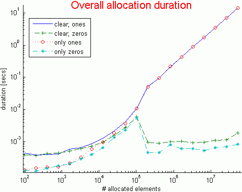
The full results were (R2013a, Win 7 64b, 8MB):

       n  clear,ones  clear,zeros    only ones   only zeros
========  ==========  ===========    =========   ==========
     100    0.000442     0.000384     0.000129     0.000124
     200    0.000390     0.000378     0.000150     0.000121
     400    0.000404     0.000424     0.000161     0.000151
     800    0.000422     0.000438     0.000165     0.000176
    1600    0.000583     0.000516     0.000211     0.000206
    3200    0.000656     0.000606     0.000325     0.000296
    6400    0.000863     0.000724     0.000587     0.000396
   12800    0.001289     0.000976     0.000975     0.000659
   25600    0.002184     0.001574     0.001874     0.001360
   51200    0.004189     0.002776     0.003649     0.002320
  102400    0.010900     0.005870     0.010778     0.005487
  204800    0.051658     0.000966     0.049570     0.000466
  409600    0.095736     0.000901     0.095183     0.000463
  819200    0.213949     0.000984     0.219887     0.000817
 1638400    0.421103     0.001023     0.429692     0.000610
 3276800    0.886328     0.000936     0.877006     0.000609
 6553600    1.749774     0.000972     1.740359     0.000526
13107200    3.499982     0.001108     3.550072     0.000649
26214400    7.094449     0.001144     7.006229     0.000712
52428800   14.039551     0.001853    14.396687     0.000822
(Note: all numbers should be divided by the number of loop iterations iters=100)
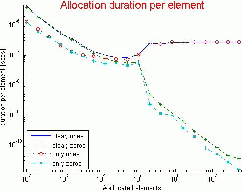
As can be seen from the data and resulting plots (log-log scale), the more elements we allocate, the longer this takes. It is not surprising that in all cases the allocation duration is roughly linear, since when twice as many elements need to be allocated, this roughly takes twice as long. It is also not surprising to see that the allocation has some small overhead, which is apparent when allocating a small number of elements.
A potentially surprising result, namely that allocating 200-400 elements is in some cases a bit faster than allocating only 100 elements, can actually be attributed to measurement inaccuracies and JIT warm-up time.
Another potentially surprising result, that zeros is consistently faster than ones can perhaps be explained by zeros being able to use more efficient low-level functions (bzero) for clearing memory, than ones which needs to memset a value.
A somewhat more surprising effect is that of the clear command: As can be seen in the code, calling clear within the timed loops has no functional use, because in all cases the variable y is being overridden with new values. However, we clearly see that the overhead of calling clear is an extra 3µS or so per call. Calling clear is important in cases where we deal with very large memory constructs: clearing them from memory enables additional memory allocations (of the same or different variables) without requiring virtual memory paging, which would be disastrous for performance. But if we have a very large loop which calls clear numerous times and does not serve such a purpose, then it is better to remove this call: although the overhead is small, it accumulates and might be an important factor in very large loops.
Another aspect that is surprising is the fact that zeros (with or without clear) is much faster when allocating 200K+ elements, compared to 100K elements. This is indicative of an internal switch to a more optimized allocation algorithm, which apparently has constant speed rather than linear with allocation size. At the very same point, there is a corresponding performance degradation in the allocation of ones. I suspect that 100K is the point at which Matlab’s internal parallelization [3] (multi-threading) kicks in. This occurs at varying points for different functions, but it is normally some multiple of 20K elements (20K, 40K, 100K or 200K – a detailed list was posted [4] by Mike Croucher again). Apparently, it kicks-in at 100K for zeros, but for some reason not for ones.
The performance degradation at 100K elements has been around in Matlab for ages – I see it as far back as R12 (Matlab 6.0), for both zeros and ones. The reason for it is unknown to me, if anyone could illuminate me, I’d be happy to hear. The new thing is the implementation of a faster internal mechanism (presumably multi-threading) in R2008b (Matlab 7.7) for zeros, at the very same point (100K elements), although for some unknown reason this was not done for ones as well.
Another aspect that is strange here is that the speedup for zeros at 200K elements is ~12 – much higher than the expected optimal speedup of 4 on my quad-core system. The higher speedup may perhaps be explained by hyper-threading or SIMD [5] at the CPU level.
In any case, going back to the original reason I started this investigation, the reason for getting such wide disparity in speedups between using zeros and ones for 10K elements (as in Mike Croucher’s post), and for 3M elements (as in my pre-allocation performance article) now becomes clear: In the case of 10K elements, multi-threading is not active, and zeros is indeed only 20-30% faster than ones; In the case of 3M elements, the superior multi-threading of zeros over ones enables much larger speedups, increasing with allocated size.
Some take-away lessons:
- Using zeros is always preferable to ones, especially for more than 100K elements on Matlab 7.7 (R2008b) and newer.
zeros(n,m)+scalaris consistently faster thanones(n,m)*scalar, especially for more than 100K elements, and for the same reason.- In some cases, it may be worth to use a built-in function with more elements than actually necessary, just to benefit from its internal multi-threading.
- Never take performance assumptions for granted. Always test on your specific system using a representative data-set.
p.s. – readers who are interested in the historical evolution of the zeros function are referred to Loren Shure’s latest post [6], only a few days ago (a fortunate coincidence indeed). Unfortunately, Loren’s post does not illuminate the mysteries above.
6 Comments To "Allocation performance take 2"
#1 Comment By Joshua Leahy On August 14, 2013 @ 16:41
It’s likely that zeros becomes much faster than ones at such large sizes because matlab would switch to using mmap rather than a combination of malloc and bzero. Mmap provides you with any amount of prezeroed memory in constant time.
The trick is achieved by the operating system lazily allocating the memory on first use. If I’m right then you might see a penalty on the first use of larger allocations, but not on smaller ones.
#2 Comment By Amro On August 14, 2013 @ 17:04
Just yesterday, I was looking into a similar topic on Stack Overflow: [13]
One of the things I found while investigating the issue is that MATLAB appears to be using a custom memory allocator optimized for multi-threaded cases, namely Intel TBB scalable memory allocator (libmx.dll had a dependency on tbbmalloc.dll which is Intel’s library). I suspect that the implementation of zeros switch to this parallel memory allocator once the size is large enough.
btw there are all sorts of memory allocators out there, each claiming to be better than the others: [14]
—
I should point out that “bzero” you mentioned is now deprecated [1], and even appears to be using the same underlying call as “memset” [2]. Even the specialized “ZeroMemory” in the Win32 API is typedef’ed against “memset” [3] (which is probably optimized for your platform, whether that’s implemented in kernel code or by the CRT library).
I think the difference between zeros and ones could be explained by the performance of malloc+memset vs. calloc. There’s an excellent explanation over here: [15]
_
[1]: [16]
[2]: [17]
[3]: [18]
#3 Comment By Yair Altman On August 15, 2013 @ 11:06
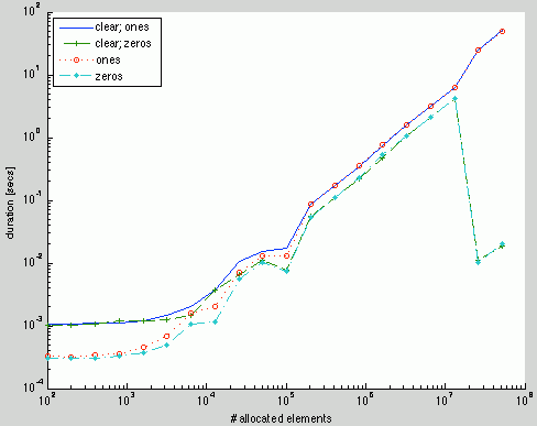
@Amro – thanks for the detailed comment and references. You may indeed be correct regarding Intel, since I’ve received the following results for a MacBook Pro (R2013a, Mountain Lion) from Malcolm Lidierth (thanks!):

#4 Comment By Michelle Hirsch On August 20, 2013 @ 07:11
Interesting assessment Yair, but it turns out that the reasons for the behavior changes aren’t what you thought. The performance change for zeros in R2008b resulted from a change in the underlying MATLAB memory management architecture at that time.
#5 Comment By Yair Altman On August 20, 2013 @ 14:36
@Michelle – thanks for the clarification
#6 Comment By Roberto On September 5, 2013 @ 08:58
The results I get from R2012b on my MacBook Pro (10.8.4) are quite different from the plot you’ve been sent. The performance of zeros and ones is practically identical for me, to the point that the two lines in the plot are practically indistinguishable (the maximum difference between the two is about 0.01 sec without normalising by the number of iterations).
Also, the time growth is linear (no improvement for 200K+ elements), which makes me wonder if R2013a introduced a new memory allocation algorithm.