Convolution performance

February 3, 2016 7 Comments

MathWorks’ latest MATLAB Digest (January 2016) featured my book “Accelerating MATLAB Performance“. I am deeply honored and appreciative of MathWorks for this.

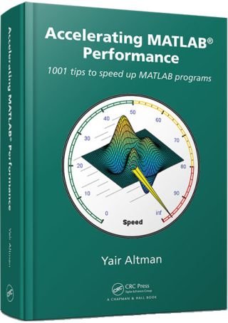
I would like to dedicate today’s post to a not-well-known performance trick from my book, that could significantly improve the speed when computing the convolution of two data arrays. Matlab’s internal implementation of convolution (conv, conv2 and convn) appears to rely on a sliding window approach, using implicit (internal) multithreading for speed.

However, this can often be sped up significantly if we use the Convolution Theorem, which states in essence that conv(a,b) = ifft(fft(a,N) .* fft(b,N)), an idea proposed by Bruno Luong. In the following usage example we need to remember to zero-pad the data to get comparable results:

% Prepare the input vectors (1M elements each)
x = rand(1e6,1);
y = rand(1e6,1);
 
% Compute the convolution using the builtin conv()
tic, z1 = conv(x,y); toc
 => Elapsed time is 360.521187 seconds.
 
% Now compute the convolution using fft/ifft: 780x faster!
n = length(x) + length(y) - 1;  % we need to zero-pad
tic, z2 = ifft(fft(x,n) .* fft(y,n)); toc
 => Elapsed time is 0.463169 seconds.
 
% Compare the relative accuracy (the results are nearly identical)
disp(max(abs(z1-z2)./abs(z1)))
 => 2.75200348450538e-10

This latest result shows that the results are nearly identical, up to a tiny difference, which is certainly acceptable in most cases when considering the enormous performance speedup (780x in this specific case). Bruno’s implementation (convnfft) is made even more efficient by using MEX in-place data multiplications, power-of-2 FFTs, and use of GPU/Jacket where available.

It should be noted that the builtin Matlab functions can still be faster for relatively small data arrays, or if your machine has a large number of CPU cores and free memory that Matlab’s builtin conv* functions can utilize, and of course also depending on the Matlab release. So, your mileage might well vary. But given the significant speedup potential, I contend that you should give it a try and see how well it performs on your specific system and data.

If you have read my book, please be kind enough to post your feedback about it on Amazon (link), for the benefit of others. Thanks in advance!

7 Responses

Alex February 28, 2016 at 19:22 Reply

Could you please provide a code for 2D version? In case of linked .mex is not working any faster than standard convolution.

Yair Altman February 28, 2016 at 21:00 Reply

@Alex – you can take a look at the m-code within Bruno’s convnfft utility for this. The speedup depends on several factors, including the size of the data, the Matlab release, and your available memory. So it is quite possible that on your specific system with your specific data you do not see significant speedup, but in many cases Bruno’s convnfft does improve the processing speed.

Alex September 30, 2017 at 16:50 Reply

Hello,

I am having a problem trying to do FFT-based convolution in 2D. convnfft is definitely the fastest one, but only imfilter produces a valid result. For convnfft and convn the result is wrong, as can be seen in the minimal working example below:

% generate image
len = 2^10;
CICcut = zeros (len);
CICcut = imnoise (CICcut, 'salt & pepper', 0.0001);
CICcut = CICcut.*(rand(len)).^2;
gauss = fspecial('gaussian', round(sqrt(len)), sqrt(sqrt(len)));
CICcut = imfilter (CICcut, gauss, 'replicate', 'conv');
 
% generate kernel
g = zeros(len);
lenMone = len-1;
for i = 1:len
    for j = 1:len
        g(i, j) = ((i-1)/lenMone - 0.5)^2 + ((j-1)/lenMone - 0.5)^2;
    end
end
g = -log(sqrt(g));
 
% convolution
tic
filtered    = imfilter (g, CICcut, 'replicate', 'conv');
toc
tic
filteredFFT = conv2fft (g, CICcut, 'same');
toc
tic
filteredN   = convn (g, CICcut, 'same');
toc
 
% display
figure('units', 'normalized', 'outerposition', [0 0.25 1 0.5])
subplot 151, imshow (CICcut, []);      title ('Mass density')
subplot 152, imshow (g, []);           title ('Green`s function')
subplot 153, imshow (filtered, []);    title ({'Gravitational potential' 'imfilter'})
subplot 154, imshow (filteredFFT, []); title ({'Gravitational potential' 'conv2fft'})
subplot 155, imshow (filteredN, []);   title ({'Gravitational potential' 'convn'})

Best regards,
Alex

Yair Altman October 1, 2017 at 17:42
@Alex – this is due to your use of the optional 'replicate' option in your call to imfilter. You are not doing the same with conv2fft or convn, which causes the results to look different. Border-pixels replication is especially important in cases such as yours where the kernel size is the same size as the input image;

If you remove the 'replicate' option in your call to imfilter, you will see that the results look the same (to the naked eye at least…).

If you want to use conv2fft or convn rather than the slow imfilter, and yet you still want to see a nice-looking image, then you should either reduce the kernel size, or enlarge the input image (so that the original image is at its center) and take care of the boundary pixels. You can either do it the same way as the 'replicate' option, or in a different way. For example, here is a simple implementation that at least in my eyes gives superior results even compared to imfilter:
c2 = repmat(CICcut,3,3); % c2 is 3072x3072, CICcut is 1024x1024 filteredN = convn (g, c2, 'same'); subplot 155, imshow (filteredN, []); title ({'Gravitational potential' 'convn'})
c2 = repmat(CICcut,3,3); % c2 is 3072x3072, CICcut is 1024x1024 filteredN = convn (g, c2, 'same'); subplot 155, imshow (filteredN, []); title ({'Gravitational potential' 'convn'})

Jackie Shan September 6, 2016 at 01:27 Reply
When looking at the CPU utilization, I noticed that the ND convolution function (convn) does not use multiple cores when operating on greater than 2D arrays.
A=randn(500,500); B=randn(500,500); C=convn(A,B,'same'); % all 12 CPUs are utilized A=randn(500,50,10); B=randn(500,50,10); C=convn(A,B,'same'); % only 1 CPU is utilized
A=randn(500,500); B=randn(500,500); C=convn(A,B,'same'); % all 12 CPUs are utilized A=randn(500,50,10); B=randn(500,50,10); C=convn(A,B,'same'); % only 1 CPU is utilized
I was wondering if there’s any reason for this?

Yair Altman September 6, 2016 at 10:12 Reply

@Jackie – I believe this is due to a sub-optimal implementation. MathWorks has limited engineering resources and probably decided that 2D convolution is much more common than 3D. I assume that MathWorks focused its engineers on improving the performance of the 2D case and then moved on to more pressing matters, instead of also solving the harder and less-used 3D case. In a world with limited resources this is certainly understandable.

Coo Coo December 6, 2022 at 22:26 Reply

FFT-based convolution is circular whereas MATLAB’s conv functions have several options (‘valid’, ‘same’, ‘full’) but unfortunately not ‘circ’. For that you need to wrap your own conv function at a cost of replicating the array with padding.

function C = cconvn(A,B)
% cconvn  N-dimensional circular convolution
 
sA = size(A);
sB = size(B);
 
% indices with wrapped endpoints
for k = 1:numel(sA)
    if sA(k)==1 || k > numel(sB) || sB(k)==1
        s{k} = ':';
    else
        s{k} = [sA(k)-ceil(sB(k)/2)+2:sA(k) 1:sA(k) 1:floor(sB(k)/2)];
    end
end
 
% pad array for convn valid
C = convn(A(s{:}),B,'valid');

HTML tags such as <b> or <i> are accepted.
Wrap code fragments inside <pre lang="matlab"> tags, like this:

<pre lang="matlab">
a = magic(3);
disp(sum(a))
</pre>

I reserve the right to edit/delete comments (read the site policies).
Not all comments will be answered. You can always email me (altmany at gmail) for private consulting.

Click here to cancel reply.

Related posts:

7 Responses

Leave a Reply