Pinning annotations to graphs

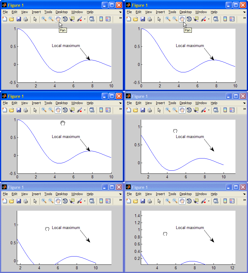
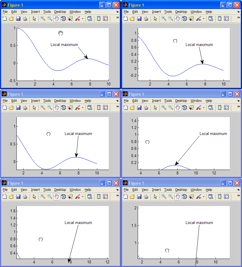
Many Matlab users are aware of Matlab’s annotation functionality, which enables us to assign graphic elements such as arrows, lines, ellipses and text labels to Matlab figures. Matlab has a corresponding built-in function, annotation, that enables creation of annotation objects. Through the handle returned by annotation we can customize the annotation’s appearance (for example, line width/style or text font properties).

Limitations of Matlab annotations

Unfortunately, annotation has several major deficiencies, that are in fact related:

1. annotation requires us to specify the annotation’s position in normalized figure units. Often, we are interested in an annotation on a plot axes that does NOT span the entire figure’s content area. To correctly convert the position from plot axes data coordinates to figure coordinates requires non-trivial calculations.
2. The created annotation is NOT pinned to the plot axes by default. This means that the annotation retains its relative position in the figure when the plot is zoomed, panned or rotated. This results in unintelligible and misleading annotations. We can indeed pin the annotation to the graph, but this requires delicate manual interaction (click the Edit Plot toolbar icon, then right-click the relevant annotation end-point, then select “Pin to Axes” from context menu). Unfortunately, the annotation handle does not provide a documented way to do this programmatically.
3. Finally, the annotation objects are only displayed on top of plot axes – they are obscured by any GUI uicontrols that may happen to be present in the figure.

All of these limitations originate from the underlying implementation of annotation objects in Matlab. This is based on a transparent hidden axes that spans the entire figure’s content area, on which the annotations are being drawn (also called the scribe layer). The annotations may appear to be connected to the plot axes, but this is merely a visual illusion. In fact, they are located in a separate axes layer. For this reason, annotation requires figure position – in fact, the annotation has no information about the axes beneath it. Since plot axes are always obscured by uicontrols, so too is the annotation layer.
Matlab’s implementation of annotation is an attempt to replicate Java’s standard glass-pane mechanism. But whereas the Java glass-pane is a true transparent layer, on top of all other window components (examples), Matlab’s implementation only works for axes.
Oh well, it’s better than nothing, I guess. But still, it would be nice if we could specify the annotation in graph (plot axes) data units, and have it pinned automatically without requiring manual user interaction.

Debugging the problem

The obvious first place to start debugging this issue is to go to the annotation handle’s context-menu (accessible via the UIContextMenu property), drill down to the “Pin” menu item and take a look at its callback. We could then use the hgfeval function to execute this callback programmatically. Unfortunately, this does not work well, because the context-menu is empty when the annotation is first created. A context-menu is only assigned to the annotation after the Edit Plot toolbar button and then the annotation object are clicked.
Being too lazy in nature to debug this all the way through, I opted for an easier route: I started the Profiler just prior to clicking the context-menu’s “Pin to Axes”, and stopped it immediately afterwards. This showed me the code path (beneath %matlabroot%/toolbox/matlab/scribe/), and placing breakpoints in key code lines enabled me to debug the process step-by-step. This in turn enabled me to take the essence of the pinning code and implement it in my stand-alone application code.
Believe me when I say that the scribe code is complex (anyone say convoluted?). So I’ll spare you the gruesome details and skip right to the chase.

The solution

Positioning the annotation in axes data units

The first step is to ensure that the initial annotation position is within the figure bounds. Otherwise, the annotation function will shout. Note that it is ok to move the annotation outside the figure bounds later on (via panning/zooming) – it is only the initial annotation creation that must be within the figure bounds (i.e., between 0.0-1.0 in normalized X and Y units):

% Prepare the annotation's X position
% Note: we need 2 X values: one for the annotation's head, another for the tail
x = [xValue, xValue];
xlim = get(hAxes,'XLim');
% Prepare the annotation's Y position
% Note: we need 2 Y values: one for the annotation's head, another for the tail
% Note: we use a static Y position here, spanning the center of the axes.
% ^^^^  We could have used some other Y data value for this
yLim = get(hAxes,'YLim');
y = yLim(1) + 0*sum(yLim) + [0.1,0]*diff(ylim);  % TODO: handle reverse, log Y axes
% Ensure that the annotation fits in the window by enlarging
% the axes limits as required
if xValue < xlim(1) || xValue > xlim(2)
    hold(hAxes,'on');
    plot(hAxes,xValue,y(2),'-w');
    drawnow;
    % YLim may have changed, so recalculate y
    yLim = get(hAxes,'YLim');
    y = yLim(1) + 0*sum(yLim) + [0.1,0]*diff(ylim);  % TODO: handle reverse, log Y-axes
end

Next, we convert our plot data units, in order to get the annotation’s requested position in the expected figure units. For this we use %matlabroot%/toolbox/matlab/scribe/@scribe/@scribepin/topixels.m. This is an internal method of the scribepin UDD class, so in order to use it we need to create a dummy scribepin object. topixels then converts the dummy object’s position from axes data units to pixel units. We then use the undocumented hgconvertunits function to convert from pixel units into normalized figure units:

% Convert axes data position to figure normalized position
% uses %matlabroot%/toolbox/matlab/scribe/@scribe/@scribepin/topixels.m
scribepin = scribe.scribepin('parent',hAxes,'DataAxes',hAxes,'DataPosition',[x;y;[0,0]]');
figPixelPos = scribepin.topixels;
hFig = ancestor(hAxes,'figure');
figPos = getpixelposition(hFig);
figPixelPos(:,2) = figPos(4) - figPixelPos([2,1],2);
figNormPos = hgconvertunits(hFig,[figPixelPos(1,1:2),diff(figPixelPos)],'pixels','norm',hFig);
annotationX = figNormPos([1,1]);
annotationY = figNormPos([2,2]) + figNormPos(4)*[1,0];

Pinning the annotation to the axes data

Finally, we use the annotation handle’s pinAtAffordance() method and set the Pin.DataPosition property to the requested X,Y values (we need to do both of these, otherwise the annotation will jump around when we zoom/pan):

% Ensure that the annotation is within the axes bounds, then display it
if any([annotationX,annotationY] < 0) || any([annotationX,annotationY] > 1)
    % Annotation position is outside axes boundaries, so bail out without drawing
    hAnnotation = handle([]);
elseif ~isempty(annotationObj)
    % Create a text-arrow annotation with the requested string at the requested position
    hAnnotation = handle(annotation('textarrow', annotationX, annotationY, ...
                                    'String',annotationStr, 'TextColor','b', 'Tag','annotation'));
    % Example for setting annotation properties
    hAnnotation.TextEdgeColor = [.8,.8,.8];
    % Pin the annotation object to the required axes position
    % Note: some of the following could fail in certain cases - never mind
    try
        hAnnotation.pinAtAffordance(1);
        hAnnotation.pinAtAffordance(2);
        hAnnotation.Pin(1).DataPosition = [xValue, y(1), 0];
        hAnnotation.Pin(2).DataPosition = [xValue, y(2), 0];
    catch
        % never mind - ignore (no error)
    end
end

p.s. Notice that all this relies on pure Matlab code (i.e., no mention of the dreaded J-word…). In fact, practically the entire scribe code is available in m-file format in the base Matlab installation. Masochistic readers may find many hours of pleasure sifting through the scribe code functionality for interesting nuggets such as the one above. If you ever find any interesting items, please drop me an email, or post a comment below.

Undocumented annotation properties

Annotation objects have a huge number of undocumented properties. In fact, they have more undocumented properties than documented ones. You can see this using my uiinspect or getundoc utilities. Here is the list for a simple text-arrow annotation, such as the one that we used above:

>> getundoc(hAnnotation)
ans =
              ALimInclude: 'on'
                   Afsize: 6
          ApplicationData: [1x1 struct]
                 Behavior: [1x1 struct]
              CLimInclude: 'on'
               ColorProps: {5x1 cell}
     EdgeColorDescription: 'Color'
        EdgeColorProperty: 'Color'
                  Editing: 'off'
                EraseMode: 'normal'
     FaceColorDescription: 'Head Color'
        FaceColorProperty: 'HeadColor'
             FigureResize: 0
            HeadBackDepth: 0.35
                HeadColor: [0 0 0]
            HeadColorMode: 'auto'
            HeadEdgeColor: [0 0 0]
            HeadFaceAlpha: 1
            HeadFaceColor: [0 0 0]
               HeadHandle: [1x1 patch]
         HeadHypocycloidN: 3
            HeadLineStyle: '-'
            HeadLineWidth: 0.5
               HeadRosePQ: 2
                 HeadSize: 10
             HelpTopicKey: ''
          IncludeRenderer: 'on'
                 MoveMode: 'mouseover'
                    NormX: [0.2 0.4]
                    NormY: [0.5 0.7]
                      Pin: [0x1 double]
                   PinAff: [1 2]
           PinContextMenu: [2x1 uimenu]
                PinExists: [0 0]
              PixelBounds: [0 0 0 0]
        PropertyListeners: [8x1 handle.listener]
        ScribeContextMenu: [9x1 uimenu]
                 Selected: 'off'
             Serializable: 'on'
                ShapeType: 'textarrow'
                    Srect: [2x1 line]
           StoredPosition: []
                TailColor: [0 0 0]
               TailHandle: [1x1 line]
            TailLineStyle: '-'
            TailLineWidth: 0.5
     TextColorDescription: 'Text Color'
            TextColorMode: 'auto'
        TextColorProperty: 'TextColor'
        TextEdgeColorMode: 'manual'
            TextEraseMode: 'normal'
               TextHandle: [1x1 text]
         UpdateInProgress: 0
    VerticalAlignmentMode: 'auto'
              XLimInclude: 'on'
              YLimInclude: 'on'
              ZLimInclude: 'on'